Geolocating photos from the SLV's Committee for Urban Action collection
Concerned about the loss of built heritage in the 1970s, the Committee for Urban Action photographed streetscapes across urban and regional Victoria. They compiled a remarkable collection of photographs that is now being digitised by the State Library of Victoria. More than 20,000 images are already available online!
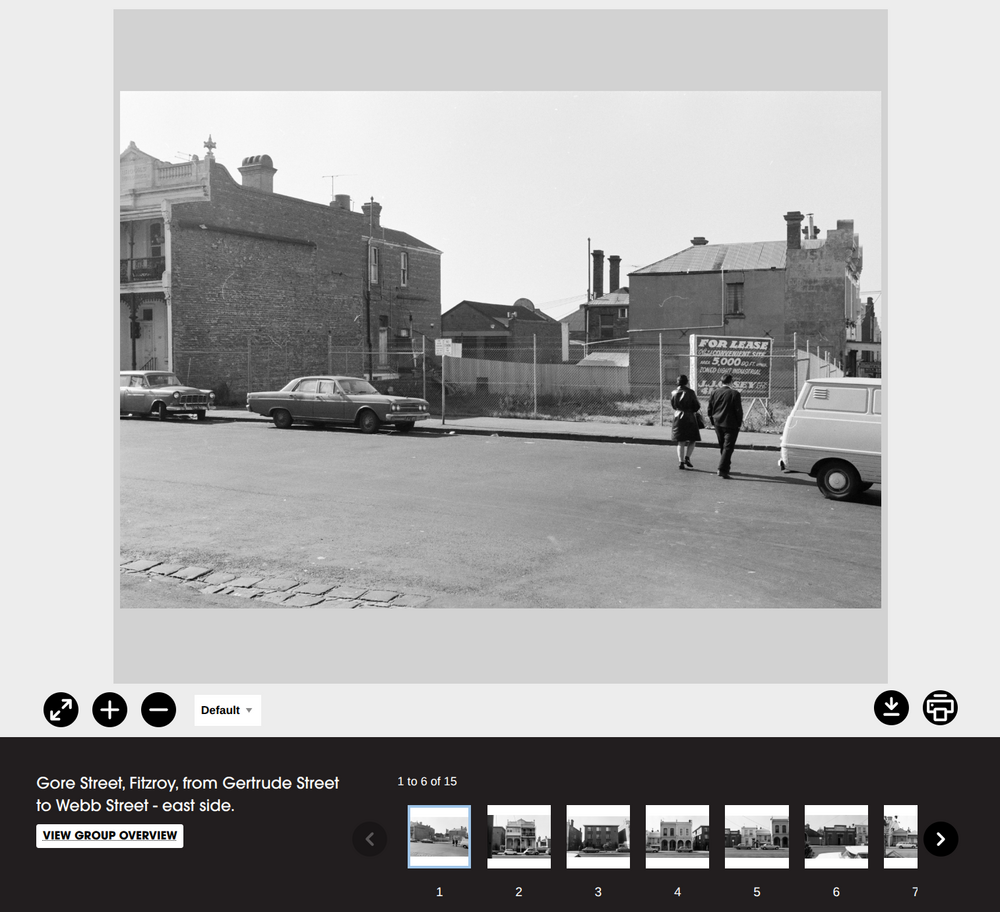
The CUA worked systematically, capturing photos street by street, and recording the locations of each set of photographs. This information is used to prepare the title attached to each photo as it’s uploaded to the SLV catalogue. In general, titles include the name of the road where the photo was taken, the name of the suburb or town, and the names of two intersecting roads that define the boundaries of the current road segment. They can also tell you which side of the road the photo was taken on. For example, the title Gore Street, Fitzroy, from Gertrude Street to Webb Street - east side tells us the photo was taken on the east side of Gore Street, Fitzroy between the intersections with Gertrude Street and Webb Street.
It’s great to have this sort of structured information linking photos to specific locations, but to navigate through the collection in space we need more. We need to link each photo to a set of geospatial coordinates by mapping each road segment. That was the challenge I took on as part of my residency in the SLV LAB.
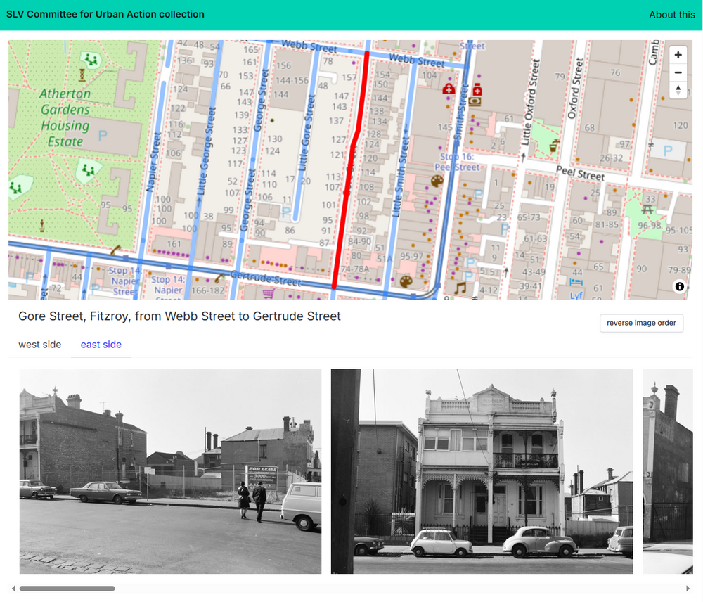
When I started working on the collection I wasn’t really sure what was possible. I had to learn a lot, and ended up revising my processes multiple times as I got deeper into the data. But my aim was always to create some sort of map-based interface, that would allow users to click on a street and see any associated CUA photos. It’s still a bit buggy and incomplete, but here it is – explore the CUA collection street by street!
The process
My basic plan was to find the intersections using OpenStreetMap, then extract geospatial information about the segment of road between the two intersections. This involved much trial and error, but eventually I ended up with a process that:
- parsed each item title to try and extract the names of the main road, the suburb, and the two intersecting roads
- queried Nominatim for the suburb bounding box
- for each intersecting road, queried OSM to find a node at, or around, its intersection with the main road, within the suburb bounding box
- created a new bounding box from the coordinates of the two intersections
- queried OSM for the main road within this bounding box
- extracted the coordinates of the main road segment, removing any points outside of the bounding box
There’s more details below and in these notebooks: cua_finding_intersections.ipynb and cua_data_processing.ipynb.
Finding intersections
As described, the title of each photograph generally includes 4 pieces of information: the road, suburb, intersecting roads, and side. My plan was to find the intersections first to get the limits of the road segment. This is possible thanks to the awesome OpenStreetMap and its Overpass API. It took me a while to get my head around the Overpass query language, but there are lots of useful examples online. The query to find the intersection between Gore Street and Gertrude Street in Fitzroy looks like this:
[bbox:-37.8089071,144.9732006,-37.7929130,144.9851430];
way['highway'][name="Gore Street"];
node(w)->.n1;
way['highway'][name="Gertrude Street"];
node(w)->.n2;
node.n1.n2;
out body;
You can try it out using Overpass Turbo’s web interface.
In OpenStreetMap, linear features, such as roads or rivers, are represented as ways. Each way is made up of a series of nodes or points with geospatial coordinates. Every way and node has its own unique identifier. Tags can be added to features to describe what type of things they are.
The query above looks for ways named ‘Gore Street’ and ‘Gertrude Street’ that are tagged as highway (a highway in OpenStreetMap is any road-like feature including things bike paths and foot trails).
way['highway'][name="Gore Street"];
It then extracts the nodes that make up each way and looks to see if there are any nodes in common between the two ways. A node shared between two ways indicates an intersection.
node(w)->.n2;
node.n1.n2;
The query is limited using a bounding box that encloses the suburb of Fitzroy. This avoids false positives and keeps down the query load.
[bbox:-37.8089071,144.9732006,-37.7929130,144.9851430];
The JSON result of this query gives as the latitude and longitude of the node at the intersection of the two roads.
{
  "version": 0.6,
  "generator": "Overpass API 0.7.62.10 2d4cfc48",
  "osm3s": {
    "timestamp_osm_base": "2026-01-27T03:11:45Z",
    "copyright": "The data included in this document is from www.openstreetmap.org. The data is made available under ODbL."
  },
  "elements": [

{
  "type": "node",
  "id": 224750459,
  "lat": -37.8062302,
  "lon": 144.9817848
}

  ]
}
After a bit of testing, I found this worked pretty well, except for roundabouts… In OpenStreetMap, roads don’t actually cross roundabouts – they end on one side, then begin anew on the other side. In cases like this, looking for shared nodes doesn’t work. Instead you have to look to see if the two roads have nodes that are less than a given distance apart. The query is similar to the one above, but uses around when comparing the nodes. In this case I’m looking for nodes that are within 20 metres of each other.
node(w.w2)(around.w1:20);
Finding road segments
Once I had the coordinates of the two intersections, I could look for the segment of road between between them. To do this I created a bounding box using the coordinates of the intersections, and then searched for ways by name within that defined area.
It’s important to note that there’s no one-to-one correspondence between roads and OSM ways. A single road might be represented in OSM as a series of separate, but connected, ways. For example, at a roundabout, or where a road divides, new ways might have been created to document the change. This means that when we query OSM for details of a road we often get back information about multiple ways. Some of these might be things like bike paths which we can filter using tags, but often they’ll be sections of the road that we want. For example, this query for Gore Street, within the bounds of its intersections with Gertrude Street and Webb Street, returns details of two ways.
way["highway"~"^(trunk|primary|secondary|tertiary|unclassified|residential|service|track|pedestrian|living_street)$"][name="Gore Street"](-37.8062302,144.98128480000003,-37.8040076,144.9826827);
out body;
>;
out body;
You can view the result in Overpass Turbo.
However, that doesn’t mean that the full extent of both ways is contained within the bounding box, just that some of the nodes of both ways are inside. Because of this, I filtered the results from all the ways and only kept nodes whose coordinates were within the desired region.
Problems finding intersections
The method described above works pretty well, and once I understood enough about the Overpass API to get out actual paths that I could display on a map, I fed all of the CUA photos through a script and got useful data for more than 80% of them.
Then I spent a lot of time trying to understand where the remainder were failing.
Some of them failed because the titles were missing information, or were formatted in a way I didn’t expect. For example, instead of a second intersecting road, some titles just said ‘to end’. This makes perfect sense to a human looking at a map, but it’s difficult to handle programmatically.
Some photos either recorded the wrong suburb, or the boundaries of the suburb had moved since the photos were taken. For example, many of the photos described as being from Eaglehawk are now in California Gully.
Similarly, some road names were wrong either because of documentation errors, or because the names have changed over time. There are also some variations in the way OSM records road names – in particular, I found that roads with hyphenated names sometimes had spaces around the hyphen and sometimes didn’t. There were also a couple of cases where names weren’t attached to the corresponding road segment in OSM, but I was able to edit these in OSM directly.
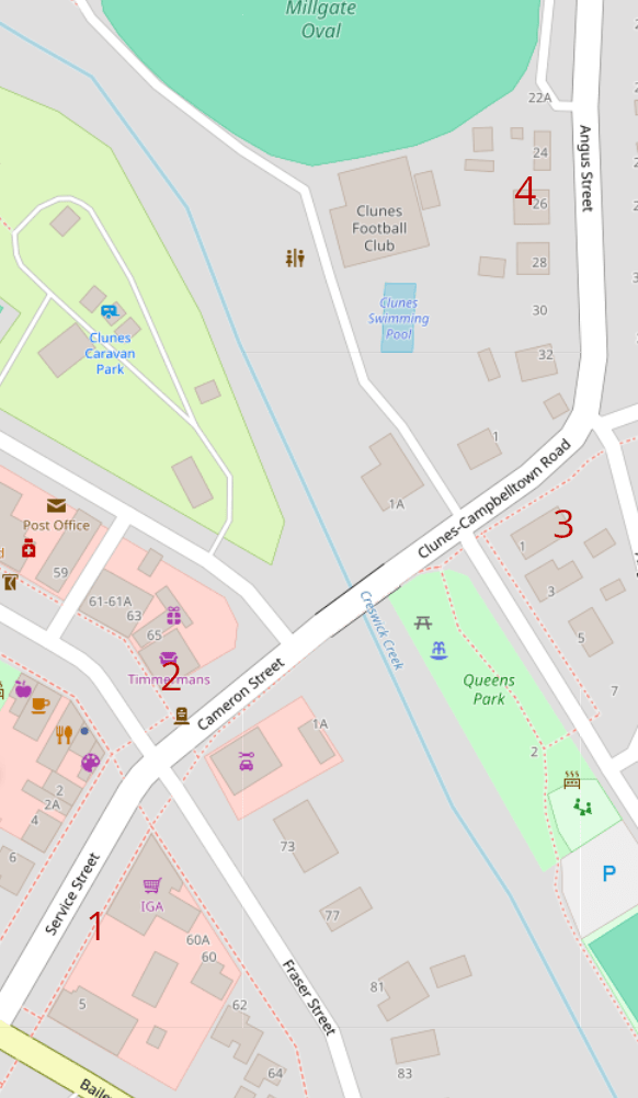
Other roads had multiple names, or change names along their path. I mean, what’s going on with Brunswick Street and St Georges Road in Fitzroy? Country towns seemed most prone to this – a highway might become ‘Main Road’ within the town boundaries, or the order of hyphenated places in road names might change. I found one road in Clunes that had four different names within the space of a few hundred metres.
Finally, the routes of some roads had changed – intersections no longer intersected, roads were closed, or new parks had popped up to split a road in two.
My processing script logged the titles I couldn’t locate and I worked through the list manually, trying to identify what each problem was. I suppose there’s two ways I could’ve handled these problems – building more fuzziness into the process to check for things like alternative names, or by compiling a list of ‘corrected’ titles. I started off using the first approach, but as I worked through more and more anomalies, the checking logic became very complicated and inefficient. Just think about the knots you can tie yourself in trying to handle a title where the suburb is wrong and the main road changes names in between intersections.
I refactored the code multiple times, but it’s still pretty messy. In the end I created a list of ‘corrected’ titles as well, so it was a bit of a hybrid approach. I suspect I could have saved myself a lot of pain if I’d reversed the process – compiling ‘corrected’ titles first, then adapting the logic as patterns emerged.
There are still some photos I haven’t located. In some cases I just don’t have enough information. In others I need to manually record coordinates or way ids to feed into the process, and I haven’t worked out the best way to do this yet. You can see the titles that I’ve haven’t geolocated yet in the files: cua-not-found.txt and cua-not-parsed.txt.
In total, 18,603 out of 20,644 photos have been geolocated. That’s over 90%!
Assembling the data
I processed the data in a couple of phases to get it in the shape I wanted.
The first step was to group all the photos by title, so I could link each group to its location. But remember that titles often record which side of the road a photo was taken on. To bring all sides of a road segment together into a single group, I created a key from a normalised/slugified version of the title with the side value removed. I used this key to save information about each side within the same group.
I ended up with a dataset with this sort of structure (a truncated example):
"iffla-street-south-melbourne-coventry-street-normanby-street":
    {
        "title": "Iffla Street, South Melbourne, from Coventry Street to Normanby Street",
        "sides":
        {
            "east side":
            {
                "title": "Iffla Street, South Melbourne, from Coventry Street to Normanby Street - east side.",
                "images":
                [
                    {
                        "ie_id": "IE20321667",
                        "alma_id": 9939649155207636
                    }
                    more photos...
                ]
            },
            "west side":
            {
                "title": "Iffla Street, South Melbourne, from Normanby Street to Coventry Street - west side.",
                "images":
                [
                    {
                        "ie_id": "IE20320072",
                        "alma_id": 9939655629407636
                    },
					more photos...
                ]
            }
        },
        "ways":
        {
            "27631235":
            [
                [
                    144.9503379,
                    -37.835322
                ],
                more points...
            ]
        }
    },
You can see how the sides and matching ways have been brought together under the key value.
This structure was useful for grouping and processing the data, but to create a map interface I needed to bring the geospatial information to the surface. The first version of the interface used one big GeoJSON file in which the features were MultiLineStrings created from the paths of each road segment. The photo data was saved in the properties of each GeoJSON feature.
It sort of worked. The roads with photos were highlighted, and clicking on the roads displayed the photos. It was only when I changed the opacity of the lines that I realised that, in many cases, different road segments were being piled on top of each other. When the lines were opaque these piles were invisible, but add a bit of transparency and you could see that some lines were darker than others. Clicking on the lines only displayed the top layer, so some groups of photos were effectively invisible.
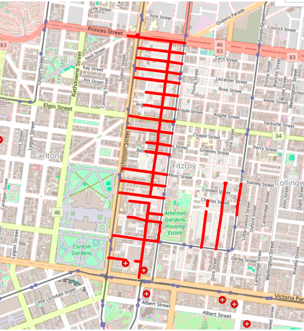
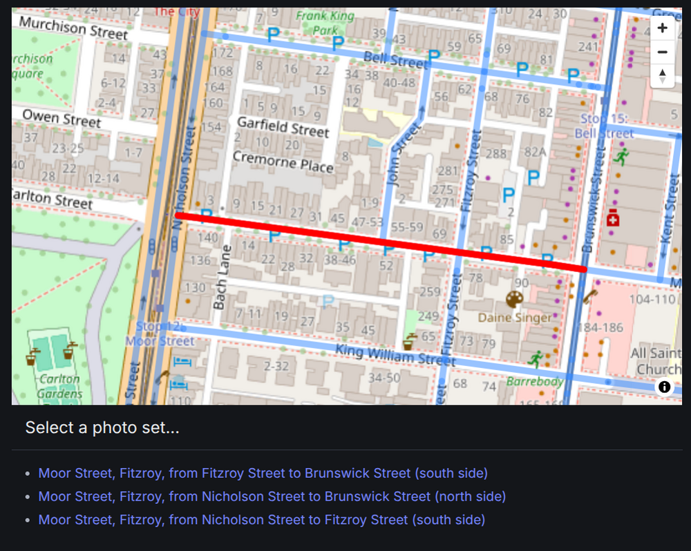
Why did this happen? I’d wrongly assumed that each segment of road would only have one group of photos associated with it. But it’s not hard to find cases where this is not true. Consider Moor Street, Fitzroy, between Nicholson Street and Brunswick Street. On the north side, there is a single group of photos that document the buildings between Nicholson Street and Brunswick Street. However, on the south side there’s two groups of photos. One covers the section between Nicholson Street and Fitzroy Street, the other covers Fitzroy Street to Brunswick Street. One section of road, three groups of photos…
To make these layered groups more easily accessible through the interface I had to change the way the data was organised – separating the GeoJSON from the photosets so that multiple photosets could be associated with a single geospatial feature. I decided to create a GeoJSON feature for every OSM way in the dataset. However, I needed to prune the way’s coordinates to only include those that were part of the CUA road segments. To do this, I saved all the way data when I found the road segments. Then in the second processing phase, I grouped the way coordinates associated with the road segments and compared this list to the full way path. Any coordinate in the way path that wasn’t in the road segments was removed. It seems unnecessarily complex, but I wanted to make sure that only the parts of roads associated with photos were highlighted in the interface.
The result was two data files. The first, cua-ways.geojson, contains the pruned way paths and their OSM identifiers. The second, cua-photos.json, contains information about each photo set, including the sides, photos, paths, and associated way identifiers. The datasets are linked by the way identifiers.
Constructing the interface
My plan for the interface was pretty simple. There’d be a map on which all the road segments associated with CUA photos were highlighted. Clicking on a highlighted section would show the photos. I wanted to display the photos as if you were scanning the streetscape, so I decided to put them all side-by-side in a gallery that scrolled horizontally.
The first version used Leaflet to display the maps and, as noted above, had some problems where there were multiple photosets associated with a segment of road.
For the second version I decided to switch to MapLibre because it seems a bit more active and up-to-date. I’d already used MapLibre in the SLV Newspapers Explorer.
The interface first loads the cua-ways.geojson file to highlight the relevant roads. When you click on one of the roads, the way id is passed to a function that looks for associated photo sets in the cua-photos.json data. If there’s only one linked photoset, then the photos are displayed. However, if there’s more than one linked photoset, they’re displayed as a list. The user then selects from the list to display the related photos.
A couple of other things happen when you click on a way or select a photoset: the colour of the selected road segment changes, and the browser url is updated with the way or photoset identifier. You can bookmark or share these urls to go directly to a specific road or photoset. There’s also a button to reverse the order of the images – they scroll left to right, but sometimes they seem to have been photographed right to left.
More information and links
-
CUA data is also used in the my place app
-
CUA code and data is in the geo-maps-residency repository
-
Code for the interface is in the slv-demo-apps repository
-
all the outcomes of my SLV residency are listed on the Experiments with the State Library of Victoria’s collections page