The State Library of Victoria holds a collection of 8,804 parish maps. As part of my residency at the SLV LAB, I’ve been poking around in the metadata.

SLV staff have geocoded many of the parish maps using the Composite Gazetteer of Australia, which provides coordinates for Victorian parishes and boroughs. These coordinates give us a point which should be roughly at the centre of each map, enabling us to visualise their locations and distribution. But how much area do they cover? To answer that question we need a bounding box that includes the coordinates of each corner of the map. We could create bounding boxes by using something like AllMaps or MapWarper to georeference each individual map, but that’s going to take a while! As a quick and dirty alternative, I wondered if it was possible to generate approximate bounding boxes from the available metadata. It seems we can!

The metadata

There are three pieces of metadata we need to construct bounding boxes:

• the latitude and longitude of the centre point
• the size of the physical map
• the scale of the map (ie how the size of the map relates to real world)

The coordinates and scale can be included in a couple of different places in the map’s MARC record. The 034 field is specifically for ‘Coded Cartographic Mathematical Data’. The relevant subfields are:

• $a: category of scale
• $b: constant ratio linear horizontal scale (this is the most likely type of scale)
• $d: westernmost longitude
• $e: easternmost longitude
• $f: northernmost latitude
• $g: southernmost latitude

If the coordinates describe a point rather than a bounding box, then $d and $e will be the same, and $f and $g will be the same.

String representations of coordinates and scale can be found in the 255 field. The relevant subfields are:

• $a: statement of scale, eg Scale [ca. 1:90,000].
• $c: statement of coordinates, eg (E 142°18'/S 37°33')

The size of the map is recorded in 300 (physical description) field under the $c (dimensions) subfield. For example: on sheet 40 x 51 cm .

The method

I started with an existing dataset downloaded from the catalogue by SLV staff. This dataset included the scale and coordinate information in the 034 field, and the coordinate string in 255$c. At first I didn’t realise that the 034 held geo data, so I separately downloaded the scale information from 255:$a in each item’s MARC record (d’oh). If the maps were digitised, I also wanted their image identifiers so I could access them through the SLV’s IIIF service. The image id from the 956$e field of the MARC record can be used to construct an IIIF manifest url, so I extracted them as well.

Once I had all the catalogue data, I had to make sure everything was in a format I could work with. The coordinates in the MARC records are recorded as degrees/minutes/seconds, so I had to convert them to decimal values. The scale factor needed to be an integer, and I needed to extract the height and width as integers from the dimensions field.

I used lat_lon_parser to convert the coordinates to decimal, but needed a bit of regex string manipulation to get the values into a format that could be parsed. Regex also came to the rescue in getting the map dimensions. All the details are in this notebook.

Creating bounding boxes

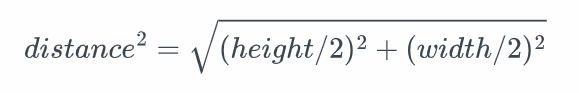
After some searching I found this StackOverflow comment that described how to create a bounding box from a point, distance, and bearing. The point I already had, but the distance and bearing had to be calculated. Trigonometry to the rescue!

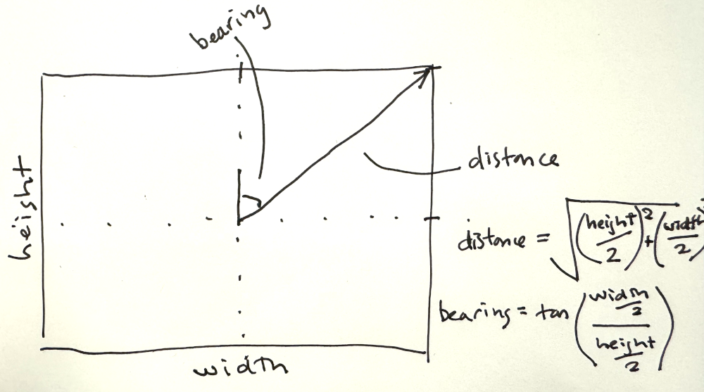
The distance from the point at the centre of the box to one of its corners is the hypotenuse of a right-angled triangle whose sides are equal to half the width and half the height of the map, and thanks to Pythagorus we know:

Once I had the distance in cm, I converted to inches, then multiplied by the scale factor, and finally converted the inches to miles. (It now occurs to me that there’s no need to convert to imperial measurements, but it doesn’t make any difference either way.)

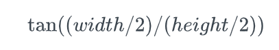
The bearing that points to the corner of the box is the angle inside the same right-angled triangle, so can be calculated using:

With the point of origin, distance, and bearing I could use geopy to calculate the corners of the bounding box!

from geopy.distance import geodesic

destination = geodesic(miles=distance).destination(origin, bearing)
coords = destination.longitude, destination.latitude

See this notebook for the full details.

Limitations

Of course, this method is very rough and has a number of major limitations, in particular:

• only about 38% of the maps have point coordinates
• the point values don’t necessarily locate the centre of the map
• not all the maps are oriented towards north
• sometimes a parish includes multiple maps
• the size of the margin around the map will affect the accuracy of the bounding box

But despite these problems the results seem pretty good. To test this I created a notebook to overlay the digitised maps on a modern basemap using the bounding boxes. Here’s an example.

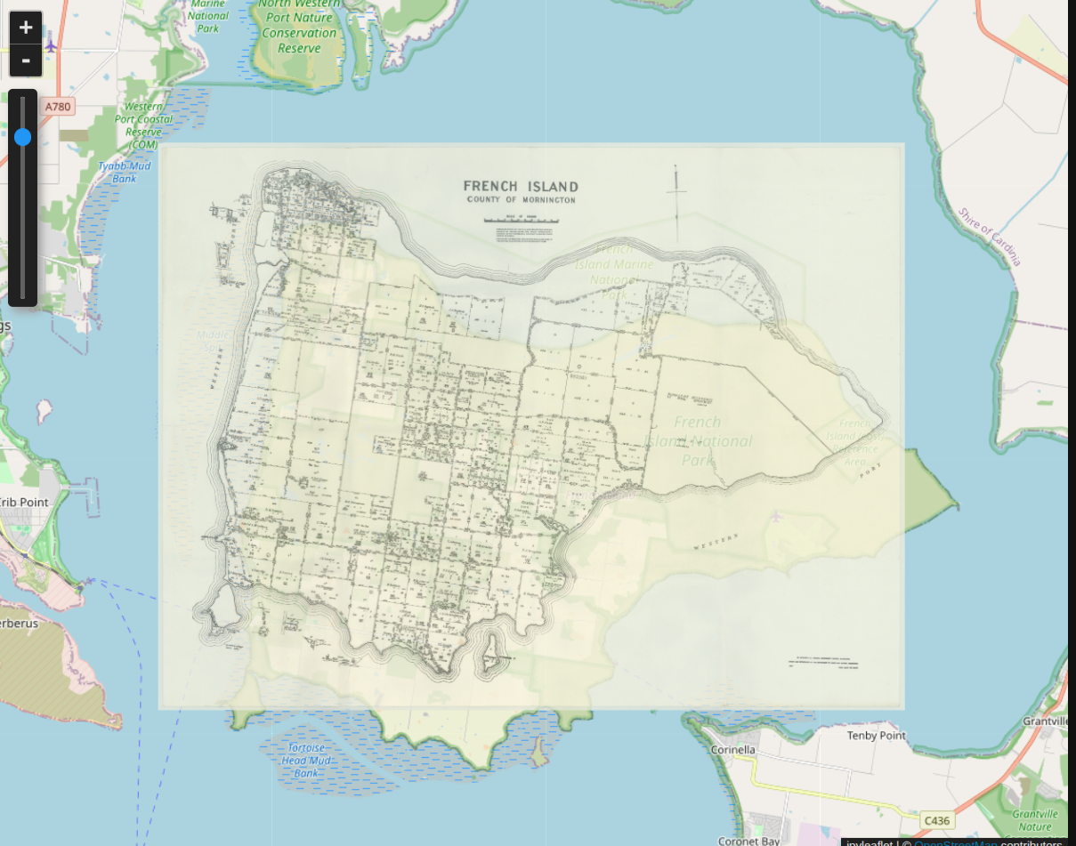
You can see the map is slightly offset (presumably due to the second problem listed above). But the size seems about right. Certainly good enough to use the bounding boxes in some exploratory analyses!

Visualising the results

I’ve saved the processed data as a new dataset, and started playing around with a couple of ways of visualising the results. These are experiments, not discovery interfaces. But you can use them for a bit of exploration if you don’t mind a few bugs. They’re all in Jupyter notebooks that can be run using the Binder service.

The parish maps browser includes a dropdown list of parish maps with point coordinates. Select a map and:

• if there’s a bounding box and an image identifier, the image of the parish map will be overlaid on the modern base map using the bounding box coordinates
• if there’s a bounding box, but no image identifier, a rectangle will be drawn on the base map showing the dimensions of the bounding box
• if there are point coordinates, but no bounding box, a marker will be placed on the base map

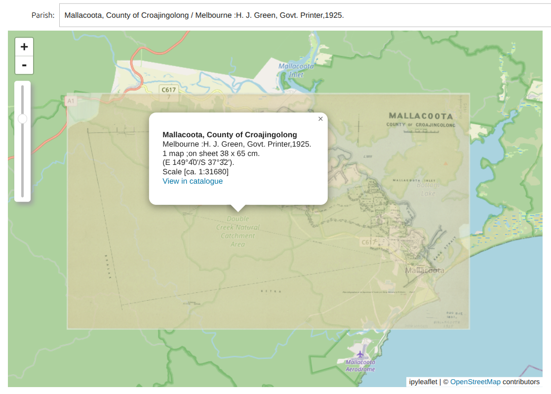
If the image of the map is displayed you can use the slider to adjust the opacity. Clicking on either the image, rectangle, or marker will display metadata about the parish map and a link to the SLV catalogue.

There’s also a visualisation of all the bounding boxes overlaid on a modern base map.

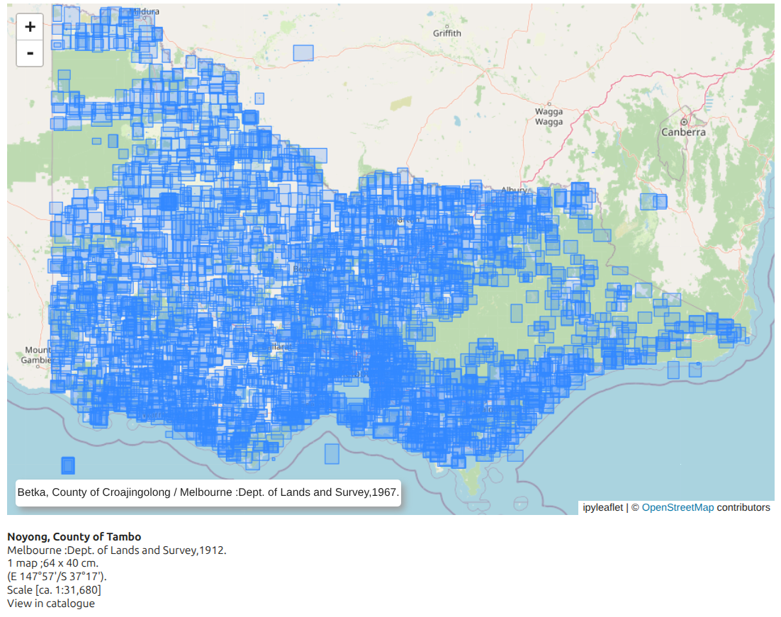
As you move your mouse over the bounding boxes the titles are displayed on the map, and if you click on a bounding box the metadata is displayed beneath the map, including a link to the SLV catalogue.

It’s obvious from the image above that some of the coordinates must be wrong! Visualisation is a great way of finding problems with your data. I now need to work through the results, documenting the problems, and thinking about how to make best use of the data. More to come!